
Metrics that drive action in Demand-Driven Manufacturing Operations
The following operations metrics put the focus on inventory management and optimizing the effectiveness of the end-to-end production process. For each metric, we designate whether it is measured at the Global (plant) or Local (resource) level.
Business value to Demand-Driven Manufacturers:
These Operations metrics help Demand-Driven Manufacturers maintain minimal inventory levels to reduce the costs associated with excess inventory and disruptions to flow.
![]()
Inventory Turns is one of the most commonly used supply chain metrics. An Inventory Turn is the number of times inventory is replaced in a given period of time. An Inventory Turn is calculated by:
Inventory Turns
= Cost of Goods Sold / Average Inventory Value
Action:
While appropriate Inventory Turns rates may vary based on industry, the following general guidance applies:
- Low Inventory Turns: First, identify the source of low inventory turns – is it demand, work in process (WIP) or raw materials?
- Demand: If the level of demand has slowed, eliminate or reduce on hand inventory.
- WIP: If you have a high level of WIP, work on improving your manufacturing processes to reduce WIP inventory.
- Raw materials: If you have high levels of finished goods or raw materials, improve your methods for determining inventory targets.
- High Inventory Turns typically signals that inventory is moving rapidly and production is flowing, indicating healthy inventory management.
Note: Because SyncManufacturing® software monitors actual usage, users of this system would measure actual Inventory Turns rather than average, or estimated turns. In this case, the calculation is:
Inventory Turns
= Actual Usage / Average Inventory Value
SyncManufacturing® software supports a comparison of Inventory Turns at the product, or item number level.
> Back to Top
![]()
Global Measurement
Cycle Time is the total amount of time it takes to complete an order – from the moment the order is released into production to the time it is completed (when the last production transaction has been recorded). This metric is valuable in identifying how much total production time (including wait time) you have in your pipeline and/or which steps in the aggregate process are longer compared to others. Cycle Time is calculated by:
Cycle time
= Time Order is Completed – Time Order is Released to Production
Action:
Monitor Cycle Time on an ongoing basis for trends. Cycle Time trending upward typically indicates a performance issue – a system bottleneck, maintenance need, etc. Cycle Times trending downward indicate effective flow; perhaps as a result of releasing a bottleneck or improving the performance of a machine.
Measuring Cycle Time can also identify variability. For example, if there is low variability in the Cycle Time for a given product, the quality of promise dates to customers will increase.
> Back to Top
![]()
Global Measurement
Queue Turns is a metric specifically associated with Demand-Driven Manufacturing that measures how often the queue turns in front of a resource over a given time period. The queue is measured by the total run and setup time (in hours) associated with the orders waiting in queue. This metric is key to flow considering that in typical environments, 85-90% of cycle time represents items waiting in the queue. A Queue Turn is calculated by:
Queue Turns
= Produced Hours / Queue Hours
Example:
If you have 50 hours of queue in front of a resource and you produce 10 hours on an average daily basis, it will take you 5 days to turn through the queue.
5 = 50 / 10
Action:
Queue Turns will be healthy if you have a good, consistent level of work flowing through production, along with a workforce that readily responds to priority orders that need to be completed.
Break down your value stream to see which work centers are turning more slowly. (This exercise may also contribute to a deeper level of analysis that can lead to improvements in Cycle Time.) A work cell with a low Queue Turn rate may point to a policy issue that indicates how your production environment is able to respond to priorities. For example, staffing levels, when and how long you run a resource, etc., could contribute to a low Queue Turn rate. A work center with low Queue Turns may also be a good candidate for your next continuous improvement event.
If Queue Turns are fluctuating for a given resource, look into the batching practices of an upstream resource as the probable culprit.
> Back to Top

Local Measurement
Schedule Adherence demonstrates the effectiveness of your manufacturing operation in working through the queue in the appropriate sequence, according to priority. That is, how well you were able to stick to the scheduled plan. Operators who work lower into the priority list and do not complete available orders of higher urgency will impact the Schedule Adherence measurement. Variations in adherence typically result in due date risks, which may affect the overall On-Time Delivery metric.
The Schedule Adherence metric is based on taking a snapshot of the queue at a particular time and comparing the completed orders at the end of the period against the available work at the time of the snapshot. If orders that were available to work on were skipped – and lower priority orders were worked on instead – then the area would not get credit for the out-of-order work completed as “good hours”. Schedule Adherence is calculated by:
Schedule Adherence Rate
= Total Produced Hours – Hours Produced out of Sequence
/ Total Produced Hours
Example:
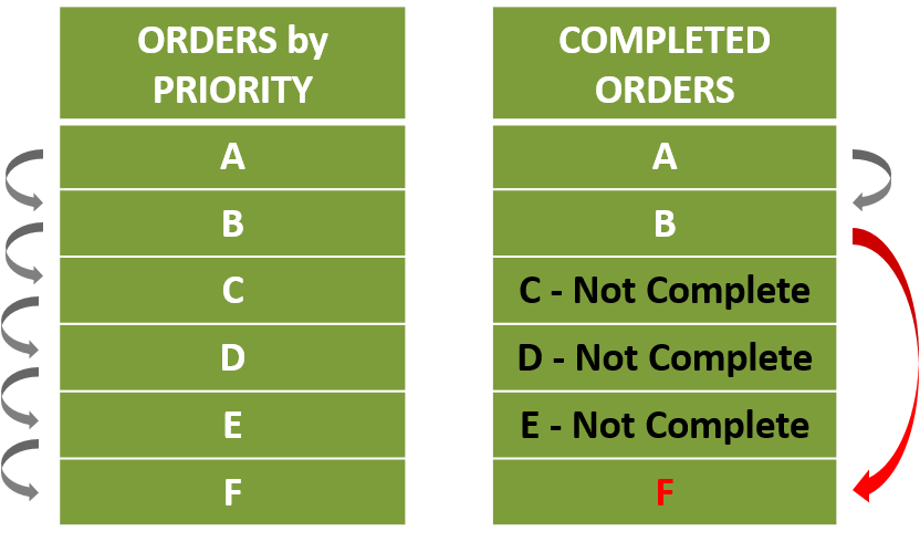
In the above example, hours for completed orders C-E would be recognized as produced out of priority and therefore the hours completed for F did not adhere to the organization’s priorities.
Note: Orders that become available to be worked within the middle of the period are also taken into account. The calculation would estimate what the priority level (and sequence within the rest of the queue) would have been at the time of the snapshot had the order been available to work. Considering this, the calculation will treat the new order like it was there over the whole period and considered accordingly.
Action:
A consequence of deviating from the scheduled plan is the negative impact to downstream production and potentially, in the ability to deliver an order on time. A sure way to drive Schedule Adherence is to measure an individual’s or cell’s performance based on this metric. As in Eli Goldratt’s famous quip, “Tell me how you will measure me and I will tell you how I will behave.”
> Back to Top

Global and Local Measurement
Demand-Driven Manufacturers manage their constraints to drive continuous flow. The Constraint Productivity metric is important in monitoring whether constraints are operating at their optimal capacity.
Constraint Productivity can be considered at both a global (plant) and local (resource) level. At the local level, the focus is on a resource constraint. At a global level, the focus is on overall throughput based on the constraint. Ultimately, the constraint is the pacemaker of the system, so by understanding the constraint productivity, you understand the flow of the entire system. Constraint Productivity is calculated by:
Constraint Productivity
= Actual Production
/ Capacity
Action:
Keep in mind that resource productivity is only valuable at the constraint resource, which is why the metric is called Constraint Productivity. A principle of Demand-Driven Manufacturing is that non-constraints do not need to have their productivity measured since they only need to be doing enough work and at a pace that will not starve constraint resources of work.
To establish this pace, identify the level of work-in-process (WIP) inventory needed to achieve optimal flow through the production process, e.g., the amount of WIP necessary to avoid starving the constraint (but no more than that). You want to get to the point where you are releasing work into production at a pace that equals the constraint resource’s production levels. This is the pace to optimize constraint productivity. (Read CONLOAD for more information.)
Commonly, measuring and therefore maximizing productivity at non-constraint resources actually has the opposite effect on overall productivity. This behavior quickly increases work-in-process (WIP), which in turn:
- Slows down the overall throughput of the factory
- Ties up more capital and cost at a given time
- Puts on-time deliveries to customers at risk
- Prevents the plant from being able to react to the most important and priority orders
> Back to Top

Global Measurement
Stock Buffer Health is the supply of inventory you keep on hand to safeguard against unforeseen demand. First, you need to have a system for indicating the status of inventory levels that represents a range of low to excess inventory. In our example and calculation, we are using red-yellow-green as our status indicators, where red equals low and green represents an overstock of inventory. Based on our example, Stock Buffer Health would be monitored based on the:
Percentage of on hand inventory items in the red, yellow and green categories.
Action:
First, create ideal inventory targets based on average levels of demand and variation. Next, establish a method for evaluating your inventory targets against actual usage. Then, monitor the percentages associated with each status level over time to identify trends. In our example, if you consistently have items in a red or green status, it indicates that your method for establishing inventory targets needs adjusting.
The following actions are based on our red-yellow-green example:
- High percentage of yellow: This is ideal and indicates a balanced level of on hand inventory.
- High percentage of green: Indicates that your inventory target is high compared to your actual usage. Trim quantity to reduce on hand waste and achieve a greater percentage of yellow.
- High percentage of red: Indicates that you are below your safety stock level and are at risk of inventory shortage. Increase the level of on hand inventory to achieve a greater percentage of yellow.
> Back to Top